
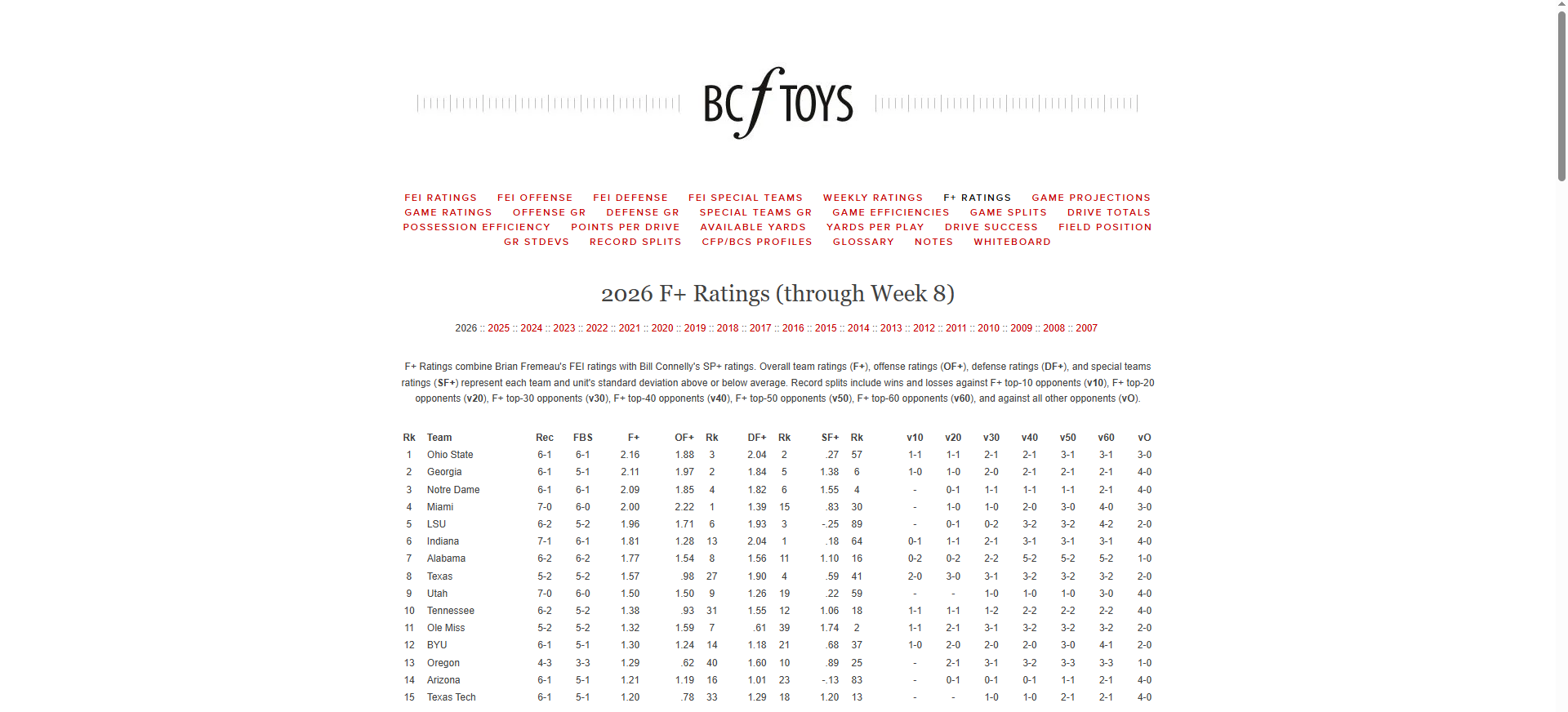
I sometimes quote F+ statistics on the College Football UK podcast, and a few listeners have asked for more details on the metric.
F+ rankings can be found at BCF Toys, alongside a whole host of other useful data. It is a composite of two other statistics, Brian Fremeau’s own FEI rating and Bill Connelly’s SP+. For true definitions from the source, you should check out their respective content pages.
What follows is my interpretation of what F+ is, why I like it and what I do with it.
The building blocks of F+
The two elements that are combined to derive F+ are as follows:
FEI – Fremeau Efficiency Index
FEI is an efficiency index which asks, “How many points per possession are a team outscoring an average opponent by, on neutral field in non-garbage time?”. It derives a scoring margin driven by who has been controlling drives more effectively.
As an example, as at week 8, Notre Dame has the highest FEI at 1.42, meaning they would theoretically outscore an average opponent by 1.42 points per possession on neutral field and in non-garbage time.
FEI is backward looking as it puts a value to what has already happened.
SP+
SP+ is a tempo and opponent adjusted efficiency index. It is expressed as an expected points per game vs an average team on a neutral field. It looks at success rate and expected points per play.
Success rate is how often teams are successful on plays. A play is considered successful if it gains: 50% of the required yards on 1st down; 70% on 2nd down; and 100% on 3rd or 4th down.
It then looks at several other factors including starting field position; points scored on drives (how they finish) and explosiveness.
Explosiveness is reflected by looking at Isolated Points per play which asks “when plays are successful, how valuable are they in earning points?”. The idea behind this is to understand if a team is slow and steady or relies on bigger chunk plays.
Ahead of week 7, Ohio State had the top SP+ rating at 26.8. So they would be expected to score this number of points per game against an average team on a neutral field.
What is F+?
If FEI is reflective of what has happened and SP+ is predictive of how things might go, F+ is the balancing item between the two.
The FEI and SP+ indexes measure and perform in different ways so it is useful to have a single metric that can even out some of those differences. Efficiency, explosiveness and success can pull in conflicting directions. You can be really efficient in moving the chains but not finish off drives with points, or not really progress drives but be bailed out by explosive chunk plays.
Therefore, F+ is an average of the other two models to give a single metric which can be used as an indicator of the overall strength of a team.
When you look at the BCF Toys webpage you will see individual unit figures for Offense, defence and special teams which are then aggregated for the total score.
How F+ is presented
To understand the F+ figure requires some understanding of statistics. I have included a section on the theory at the bottom of this article and would recommend looking at that before continuing.
Assuming you have done this, already know what you need to or are just feeling dangerous…. I will continue.
The F+ metric is presented as a statistical “z-score”. The z-score helps us measure how far away a team’s metric is from the “average team”. It standardises the “strength” metric and bases it against the average team. The unit for doing this is standard deviations.
As an example, in Week 8 Georgia had an F+ of 2.11. The average FBS team have a value of 0.
So, Georgia are 2.11 standard deviations ahead of the average team in terms of strength. That is going to put them in the top 2% of FBS teams (better than 98%).
Why is F+ useful?
Having a value based against the average (or “Mean”) allows us to look at any team relative to the average. I can look at Georgia at 2.11 and Miami at 2.00 and get a feel for how good these teams are relative to the average team at any point.
An F+ in region of 2 puts you in the top 2% of all teams (elite level). An F+ of 1 would be a considered a good team.
Rankings like the AP Top 25 poll cannot give us this difference. They cannot provide us with a sense of a team’s dominance over the rest of the field.
How do I use F+?
When I think about how strong teams are, especially when preparing my contribution to the UK media top 25 poll, I look at F+. I find it gives me a nice blended metric to answer, “how strong really are a team”. I can use this alongside looking at their strength of schedule, season record and any notable key wins.
Often, I will look at the offensive and defense F+ statistics to see how position groups match up to others.
For example, Miami has an overall F+ of 2.00 and are ranked 4th on this metric. Their offensive F+ is ranked 1st at 2.22 but their defensive F+ is ranked 15th at 1.39, a real difference between the two units. This might suggest that their success has largely been driven by the offense.
In two weeks’ time, Miami face Notre Dame who have the 4th best offensive F+ ranking at 1.85. How will the Miami defense cope against this Notre Dame offense?
I still do look at SP+ before games to think about who might win a particular game. Then, I will look at F+ for further clues on who might have the edge on either side of the ball, as well as special teams.
I also look at FEI after a game to see if a team’s performance matched what has happened in the past.
Early Limitations
It should always be remembered that both FEI and SP+ (and ultimately F+) include pre-season projected figures in the early weeks of the season. This pre-season data is phased out at different rates and to varying degrees by Brian and Bill.
Therefore, I tend to only start looking at F+ in earnest after week 6. I find this allows time for the weighting to shift towards more game data and away from pre-season projections.
Lies, damned lies, and statistics
Statistics, and especially predictive statistics, must always be treated with care.
The reality of gameday is a group of young men charging around the field doing battle. It is chaos and anything can happen.
But we know each team will get the ball around twelve times, normally for multiple plays and score (hopefully) lots of points. When this is multiplied across 138 FBS teams that is a large data set that can be used to see patterns and make some assumptions.
So yes, the stats will not always lead us to the correct conclusion, but they are useful to shape weekend narratives.
Hopefully this gives an overview on the metric and allows some of you to start using it! For me, building stories around gameday is a big part of the fun – it is even more fun if we can use some statistics to backup those stories.
Appendix – A Brief Journey into Statistics…
As mentioned above, here is a broader look at the statistical theory. I separated this section to try and keep the base article at a reasonable length!
When you collect any large pool of data (where the values are independent of each other) and plot it on a chart, it tends to follow a similar distribution pattern.
A large chunk of the values will cluster around the average (the “mean” number) and there will be fewer values that tail off in either direction.
This distribution is referred to in maths as a Normal Distribution. If you plotted all of the values in your dataset on a chart in this scenario, it would normally form a bell curve shape.
As an example, let’s say we measured a large group of people’s heights and charted them on the graph. We might end up with the below.
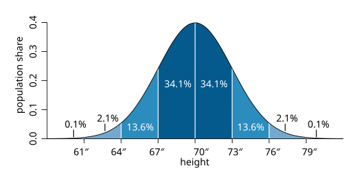
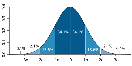
The standard deviation simply tells you how spread out the values are from the mean. The standard deviation in this example is 3.
As we can see, c68% of all values normally sit either side of 1 standard deviation from the mean. Around 95% of the values will sit within +/- 2 standard deviations of the mean.
If we have a specific data point, we can calculate its z-score, which allows us to see how many standard deviations it is away from the mean. For example, if a person in the dataset has a height of 73”, the z-score in our example is (73-70)/3 = 1 standard deviation from the mean.
Given the way the normal distribution works, we can think about the z score in terms of percentiles as follows:
-3 Standard Deviations (SD) from the mean = 0.13th percentile of all measurements
-1 SD from the mean = 16th percentile so bottom 16%
0 SD/ the mean = exactly average
1 SD from the mean = 84th percentile so better than 84%
2 SD from the mean = 98th percentile so better than 98%
3 SD from the mean = 99.87th percentile so extreme outlier
To put this in real terms in this example, a height measurement in the 98th percentile would put you in the top 2% of all measurements in the dataset.